Control of a Cart-Pole Dynamic System with TF-Agents
Reinforcement Learning (RL) to control the balancing of a pole on a moving cart
- 1. Introduction
- 2. Purpose
- 3. TF-Agents Setup
- 4. Hyperparameters
- 5. Graphical Representation of the Problem
- 6. Environment
- 7. Agent
- 8. Metrics and Evaluation
- 9. Replay Buffer
- 10. Data Collection
- 11. Training the agent
- Visualization
1. Introduction
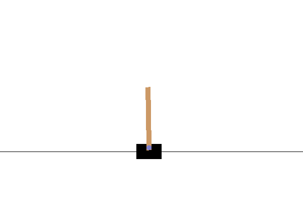
The cart-pole problem can be considered as the "Hello World" problem of Reinforcement Learning (RL). It was described by Barto (1983). The physics of the system is as follows:
- All motion happens in a vertical plane
- A hinged pole is attached to a cart
- The cart slides horizontally on a track in an effort to balance the pole vertically
- The system has four state variables:
$x$: displacement of the cart
$\theta$: vertical angle on the pole
$\dot{x}$: velocity of the cart
$\dot{\theta}$: angular velocity of the pole
Here is a graphical representation of the system:
from __future__ import absolute_import, division, print_function
import base64
import imageio
import IPython
import matplotlib
import matplotlib.pyplot as plt
import numpy as np
import PIL.Image
import pyvirtualdisplay
import tensorflow as tf
from tf_agents.agents.dqn import dqn_agent
from tf_agents.drivers import dynamic_step_driver
from tf_agents.environments import suite_gym
from tf_agents.environments import tf_py_environment
from tf_agents.eval import metric_utils
from tf_agents.metrics import tf_metrics
from tf_agents.networks import q_network
from tf_agents.policies import random_tf_policy
from tf_agents.replay_buffers import tf_uniform_replay_buffer
from tf_agents.trajectories import trajectory
from tf_agents.utils import common
tf.version.VERSION
The following is needed for rendering a virtual display:
tf.compat.v1.enable_v2_behavior()
display = pyvirtualdisplay.Display(visible=0, size=(1400, 900)).start()
NUM_ITERATIONS = 20000

INITIAL_COLLECT_STEPS = 100
COLLECT_STEPS_PER_ITERATION = 1
REPLAY_BUFFER_MAX_LENGTH = 100000

BATCH_SIZE = 64
LEARNING_RATE = 1e-3
LOG_INTERVAL = 200

NUM_EVAL_EPISODES = 10
EVAL_INTERVAL = 1000
6. Environment
Let's start with the controller. In Reinforcement Learning, the controlled entity is known as an environment. The TF-Agents framework contain some ready to use environments that can be created in TF-Agents using the tf_agents.environments suites. Fortunately, it makes access to the cart-and-pole environment (setup by OpenAI Gym) easy. Next, we load the cart-and-pole environment from the OpenAI Gym suite.
env_name = 'CartPole-v0'
env = suite_gym.load(env_name)
You can render this environment to see how it looks. A free-swinging pole is attached to a cart. The goal is to move the cart right or left in order to keep the pole pointing up. To verify, we can inspect our loaded environment with:
env.reset()
PIL.Image.fromarray(env.render())

env.action_spec()
shape specifies the structure of the input which is a scalar in this case. dtype is the data type which is an int64. The minimum value of the action is 0 and the maximum is 1. We will use the convention that the action on the cart is as follows:
-
0means LEFT -
1means RIGHT
Evolution of the Environment
The arrival of an action at the input of the environment leads to the update of its state. This is how the environment evolves. To advance the state of the environment, the environment.step method takes an input action and returns a TimeStep tuple containing the next observation of the environment and the reward for the action.
env.time_step_spec()
This specification has the following fields:
env.time_step_spec()._fields
The step_type indicates whether a step is the first step, a middle step, or the last step in an episode:
env.time_step_spec().step_type
The reward is a scalar which conveys the reward from the environment:
env.time_step_spec().reward
The discount is a factor that modifies the reward:
env.time_step_spec().discount
The observation is the observable state of the environment:
env.time_step_spec().observation
In this case we have a vector with 4 elements - one each for the cart displacement, cart velocity, pole angle, and pole angular velocity.
It is interesting to see an agent actually performing a task in an environment.
First, create a function to embed videos in the notebook.
def embed_mp4(filename):
  """Embeds an mp4 file in the notebook."""
  video = open(filename,'rb').read()
  b64 = base64.b64encode(video)
  tag = '''
  <video width="640" height="480" controls>
    <source src="data:video/mp4;base64,{0}" type="video/mp4">
  Your browser does not support the video tag.
  </video>'''.format(b64.decode())

  return IPython.display.HTML(tag)
Now iterate through a few episodes of the Cartpole game with the agent. The underlying Python environment (the one "inside" the TensorFlow environment wrapper) provides a render() method, which outputs an image of the environment state. These can be collected into a video.
def create_video(filename, action, num_steps=10, fps=30):
  filename = filename + ".mp4"
  env.reset()
  with imageio.get_writer(filename, fps=fps) as video:
    video.append_data(env.render())
    for _ in range(num_steps):
      tstep = env.step(action); print(tstep)
      video.append_data(env.render())
  return embed_mp4(filename)
action = np.array(1, dtype=np.int32) #move RIGHT action
create_video("untrained-agent", action, 50)
We are not surprised to see the pole repeatedly falling over to the left as the agent repeatedly applies an action to the right.
We will use two environments: one for training and one for evaluation.
train_py_env = suite_gym.load(env_name)
eval_py_env = suite_gym.load(env_name)
The Cartpole environment, like most environments, is written in pure Python. This is converted to TensorFlow using the TFPyEnvironment wrapper.
The original environment's API uses Numpy arrays. The TFPyEnvironment converts these to Tensors to make it compatible with Tensorflow agents and policies.
train_env = tf_py_environment.TFPyEnvironment(train_py_env)
eval_env = tf_py_environment.TFPyEnvironment(eval_py_env)
7. Agent
The controller in our problem is the algorithm used to solve the problem. In RL parlance the controller is known as an Agent. TF-Agents provides standard implementations of a variety of Agents, including:
For our problem we will use the DQN agent. The DQN agent can be used in any environment which has a discrete action space.
The fundamental problem for an Agent is how to find the next best action to submit to the environment. In the case of a DQN Agent the agent makes use of a QNetwork, which is a neural network model that can learn to predict QValues (expected returns) for all actions, given an observation from the environment. By inspecting the QValues, the agent can decide on the best next action.
fc_layer_params = (100,)
q_net = q_network.QNetwork(
    input_tensor_spec= train_env.observation_spec(),
    action_spec=       train_env.action_spec(),
    fc_layer_params=   fc_layer_params)
optimizer = tf.compat.v1.train.AdamOptimizer(learning_rate=LEARNING_RATE)
train_step_counter = tf.Variable(0)
agent = dqn_agent.DqnAgent(
    time_step_spec=     train_env.time_step_spec(),
    action_spec=        train_env.action_spec(),
    q_network=          q_net,
    optimizer=          optimizer,
    td_errors_loss_fn=  common.element_wise_squared_loss,
    train_step_counter= train_step_counter)
agent.initialize()
Policies
A policy defines the way an agent acts relative to the environment. The goal of reinforcement learning is to train the underlying model until the policy produces the desired outcome.
In this problem:
- The desired outcome is keeping the pole balanced vertically over the cart
- The policy returns an action (LEFT or RIGHT) for each
TimeStep'sobservation
Agents contain two policies:
-
agent.policy— The main policy that is used for evaluation and deployment. -
agent.collect_policy— A second policy that is used for data collection.
eval_policy = agent.policy
eval_policy
collect_policy = agent.collect_policy
collect_policy
Policies can be created independently of agents. For example, use tf_agents.policies.random_tf_policy to create a policy which will randomly select an action for each time_step.
random_policy = random_tf_policy.RandomTFPolicy(
    time_step_spec= train_env.time_step_spec(),
    action_spec=    train_env.action_spec())
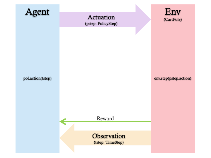
To get an action from a policy, call the policy.action(tstep) method. The tstep of type TimeStep contains the observation from the environment. This method returns a PolicyStep, which is a named tuple with three components:
-
action— the action to be taken (in this case,0or1) -
state— used for stateful (that is, RNN-based) policies -
info— auxiliary data, such as log probabilities of actions
Let's create an example environment and setup a random policy:
example_environment = tf_py_environment.TFPyEnvironment(
    suite_gym.load('CartPole-v0'))
We reset this environment:
tstep = example_environment.reset()
tstep
tstep._fields
print(tstep.step_type)
print(tstep.reward)
print(tstep.discount)
print(tstep.observation)
Now we find the PolicyStep from which the next action can be found:
pstep = random_policy.action(tstep)
pstep
pstep._fields
print(pstep.action)
print(pstep.state)
print(pstep.info)
8. Metrics and Evaluation
The most common metric used to evaluate a policy is the average return. The return is the sum of rewards obtained while running a policy in an environment for an episode. Several episodes are run, creating an average return.
The following function computes the average return of a policy, given the policy, environment, and a number of episodes.
def compute_avg_return(env, pol, num_episodes=10):
  total_return = 0.0
  for _ in range(num_episodes):
    tstep = env.reset()
    episode_return = 0.0
    while not tstep.is_last():
      pstep = pol.action(tstep)
      tstep = env.step(pstep.action)
      episode_return += tstep.reward
    total_return += episode_return
  avg_return = total_return / num_episodes
  return avg_return.numpy()[0]
# See also the metrics module for standard implementations of different metrics.
# https://github.com/tensorflow/agents/tree/master/tf_agents/metrics
Running this computation on the random_policy shows a baseline performance in the environment.
NUM_EVAL_EPISODES
compute_avg_return(eval_env, random_policy, NUM_EVAL_EPISODES)
9. Replay Buffer
The replay buffer keeps track of data collected from the environment. We will use tf_agents.replay_buffers.tf_uniform_replay_buffer.TFUniformReplayBuffer, as it is the most common.
The constructor requires the specs for the data it will be collecting. This is available from the agent using the collect_data_spec method. The batch size and maximum buffer length are also required.
replay_buffer = tf_uniform_replay_buffer.TFUniformReplayBuffer(
    data_spec=  agent.collect_data_spec,
    batch_size= train_env.batch_size,
    max_length= REPLAY_BUFFER_MAX_LENGTH)
For most agents, collect_data_spec is a named tuple called Trajectory, containing the specs for observations, actions, rewards, and other items.
agent.collect_data_spec
agent.collect_data_spec._fields
def collect_step(env, pol, buffer):
  tstep = env.current_time_step()
  pstep = pol.action(tstep)
  next_tstep = env.step(pstep.action)
  traj = trajectory.from_transition(tstep, pstep, next_tstep)
  buffer.add_batch(traj) # Add trajectory to the replay buffer

def collect_data(env, pol, buffer, steps):
  for _ in range(steps):
    collect_step(env, pol, buffer)

collect_data(train_env, random_policy, replay_buffer, INITIAL_COLLECT_STEPS)

# This loop is so common in RL, that we provide standard implementations.
# For more details see the drivers module.
# https://www.tensorflow.org/agents/api_docs/python/tf_agents/drivers
The replay buffer is now a collection of Trajectories. Let's inspect one of the Trajectories:
traj = iter(replay_buffer.as_dataset()).next()
print(type(traj))
print(len(traj))
print(traj);
traj[0]
type(traj[0])
traj[0]._fields
print('step_type:', traj[0].step_type)
print('observation:', traj[0].observation)
print('action:', traj[0].action)
print('policy_info:', traj[0].policy_info)
print('next_step_type:', traj[0].next_step_type)
print('reward:', traj[0].reward)
print('discount:', traj[0].discount)
traj[1]
type(traj[1])
traj[1]._fields
print('ids:', traj[1].ids)
print('probabilities:', traj[1].probabilities)
The agent needs access to the replay buffer. TF-Agents provide this access by creating an iterable tf.data.Dataset pipeline which will feed data to the agent.
Each row of the replay buffer only stores a single observation step. But since the DQN Agent needs both the current and next observation to compute the loss, the dataset pipeline will sample two adjacent rows for each item in the batch (num_steps=2).
The code also optimize this dataset by running parallel calls and prefetching data.
print(BATCH_SIZE)
dataset = replay_buffer.as_dataset(
    num_parallel_calls=3,
    sample_batch_size=BATCH_SIZE,
    num_steps=2).prefetch(3)
dataset
iterator = iter(dataset)
print(iterator)
NUM_ITERATIONS
# NUM_ITERATIONS = 20000
try:
  %%time
except:
  pass

# (Optional) Optimize by wrapping some of the code in a graph using TF function.
agent.train = common.function(agent.train)

# Reset the train step
agent.train_step_counter.assign(0)

# Evaluate the agent's policy once before training.
avg_return = compute_avg_return(eval_env, agent.policy, NUM_EVAL_EPISODES)
returns = [avg_return]

for _ in range(NUM_ITERATIONS):
  # Collect a few steps using collect_policy and save to the replay buffer
  collect_data(train_env, agent.collect_policy, replay_buffer, COLLECT_STEPS_PER_ITERATION)

  # Sample a batch of data from the buffer and update the agent's network
  experience, unused_info = next(iterator)
  train_loss = agent.train(experience).loss

  step = agent.train_step_counter.numpy()

  if step % LOG_INTERVAL == 0:
    print(f'step = {step}: loss = {train_loss}')

  if step % EVAL_INTERVAL == 0:
    avg_return = compute_avg_return(eval_env, agent.policy, NUM_EVAL_EPISODES)
    print(f'step = {step}: Average Return = {avg_return}')
    returns.append(avg_return)
Plots
Use matplotlib.pyplot to chart how the policy improved during training.
One iteration of Cartpole-v0 consists of 200 time steps. The environment gives a reward of +1 for each step the pole stays up, so the maximum return for one episode is 200. The charts shows the return increasing towards that maximum each time it is evaluated during training. (It may be a little unstable and not increase monotonically each time.)
iterations = range(0, NUM_ITERATIONS + 1, EVAL_INTERVAL)
plt.plot(iterations, returns)
plt.ylabel('Average Return')
plt.xlabel('Iterations')
plt.ylim(top=250)

Charts are nice. But more exciting is seeing an agent actually performing a task in an environment.
First, create a function to embed videos in the notebook.
def embed_mp4(filename):
  """Embeds an mp4 file in the notebook."""
  video = open(filename,'rb').read()
  b64 = base64.b64encode(video)
  tag = '''
  <video width="640" height="480" controls>
    <source src="data:video/mp4;base64,{0}" type="video/mp4">
  Your browser does not support the video tag.
  </video>'''.format(b64.decode())

  return IPython.display.HTML(tag)
Now iterate through a few episodes of the Cartpole game with the agent. The underlying Python environment (the one "inside" the TensorFlow environment wrapper) provides a render() method, which outputs an image of the environment state. These can be collected into a video.
def create_policy_eval_video(policy, filename, num_episodes=3, fps=30):
  filename = filename + ".mp4"
  with imageio.get_writer(filename, fps=fps) as video:
    for _ in range(num_episodes):
      time_step = eval_env.reset()
      video.append_data(eval_py_env.render())
      while not time_step.is_last():
        action_step = policy.action(time_step)
        time_step = eval_env.step(action_step.action)
        video.append_data(eval_py_env.render())
  return embed_mp4(filename)
create_policy_eval_video(agent.policy, "trained-agent")
For fun, compare the trained agent (above) to an agent moving randomly. (It does not do as well.)
create_policy_eval_video(random_policy, "random-agent")