Time-series Regression (Deep Learning to Detect Change Points)

• Purpose
• Problem
  • Change Point Detection
  • Novel approach to Change Point Detection
• Value Proposition
• Data Source
• Modeling
  • Recurrent Neural Networks (RNNs)
  • Disadvantages of RNNs
  • Time-series transformation to images
  • Convolutional Neural Networks (CNNs)
    • Convolution layers
    • Pooling layers
    • Dense layers
    • Residual Networks
• Regression Model
• Inference
• Test Dataset
• Conclusions & Recommendations
• Further Experimentation
• REFERENCES

Purpose

This project investigates whether it is feasible to use Convolutional Neural Networks (CNNs) to perform time-series regression, rather than more traditional methods. Before a CNN can be used, the time-series has to be converted to a spatial signal point, i.e. an image.

Problem

The problem for our purpose is the following: Given a time-series, detect the points in time where changes occur in the value of the time-series. The formal name for this is change point detection.

Change Point Detection

In Python, a promising package for the detection of change points, is the ruptures package by Truong, Oudre and Vayatis (2020). This package includes a number of implemented algorithms which are covered in the associated publication called "Selective review of offline change point detection methods".

The authors provide the following three highlights:

• A structured and didactic review of more than 140 articles related to offline change point detection. Thanks to the methodological framework proposed in this survey, all methods are presented as the combination of three functional blocks, which facilitates comparison between the different approaches.
• The survey provides details on mathematical as well as algorithmic aspects such as complexity, asymptotic consistency, estimation of the number of changes, calibration, etc.
• The review is linked to a Python package that includes most of the pre- sented methods, and allows the user to perform experiments and bench- marks.

... and this abstract:

This article presents a selective survey of algorithms for the offline detection of multiple change points in multivariate time series. A general yet structuring methodological strategy is adopted to organize this vast body of work. More precisely, detection algorithms considered in this review are characterized by three elements:a cost function, a search method and a constraint on the number of changes. Each of those elements is described, reviewed and discussed separately. Implementations of the main algorithms described in this article are provided within a Python package called ruptures.

This summary comes from the GitHub site:

ruptures is a Python library for off-line change point detection. This package provides methods for the analysis and segmentation of non-stationary signals. Implemented algorithms include exact and approximate detection for various parametric and non-parametric models. ruptures focuses on ease of use by providing a well-documented and consistent interface. In addition, thanks to its modular structure, different algorithms and models can be connected and extended within this package.

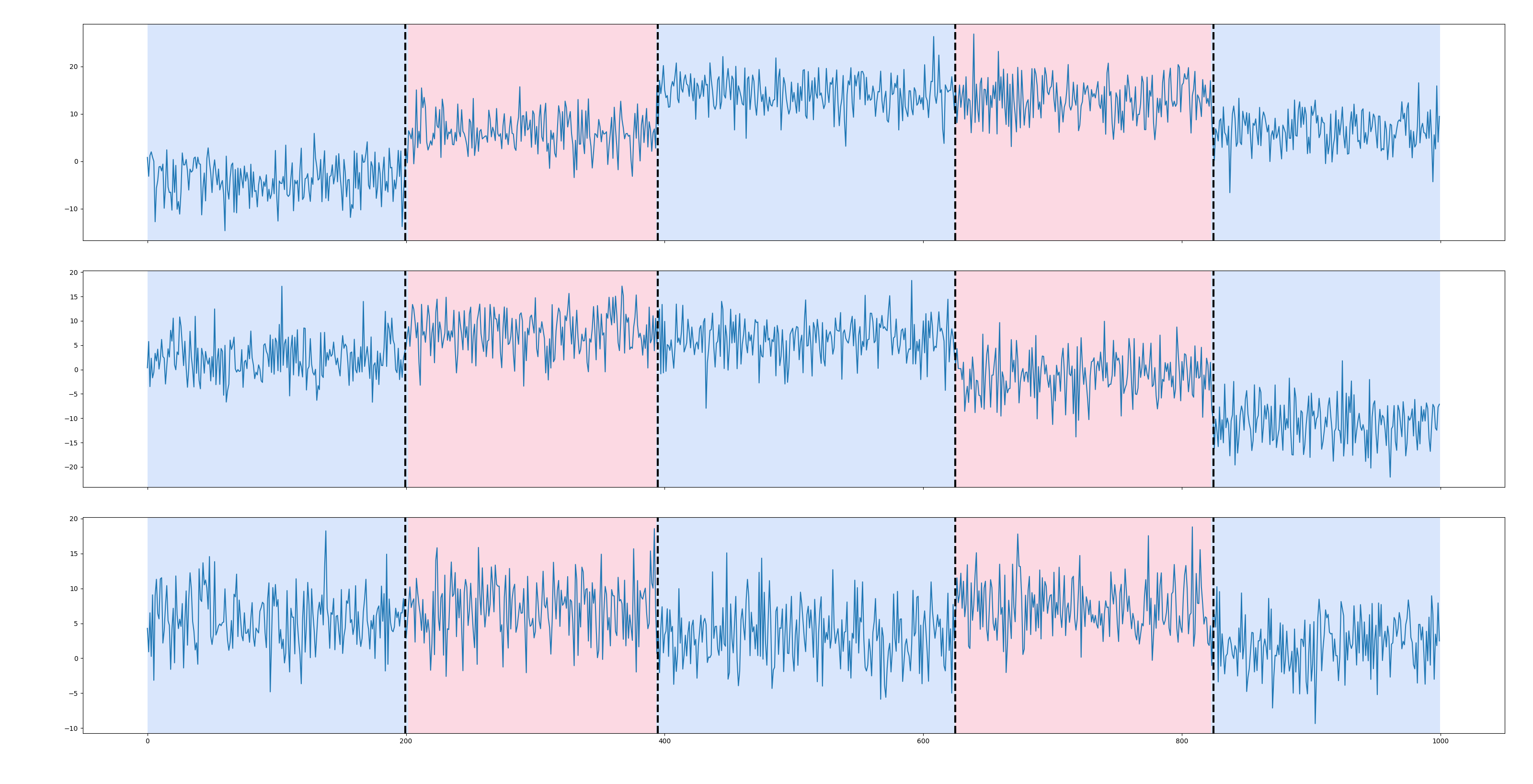
Here is an example of how the ruptures package might be used. The following code generates a noisy piecewise constant signal. Then it performs a penalized kernel change point detection and displays the results. Alternating colors outline the true regimes and vertical dashed lines mark the detected change points.

import matplotlib.pyplot as plt
import ruptures as rpt

# generate signal
n_samples, dim, sigma = 1000, 3, 4
n_bkps = 4  # number of breakpoints
signal, bkps = rpt.pw_constant(n_samples, dim, n_bkps, noise_std=sigma)

# detection
algo = rpt.Pelt(model="rbf").fit(signal)
result = algo.predict(pen=10)

# display
rpt.display(signal, bkps, result)
plt.show()

Novel approach to Change Point Detection

In the approach of this project, we do not have access to first principles models (i.e. white-box models). Instead we rely on a series of convolution neural networks (CNNs) to learn an empirical model (i.e. black-box model).

The predictor points for our problem are not structured vectors as is common in the case of structured data analysis. Here we have to use a time-series or sequence of scalar-valued predictor points and have the model learn the associated target point which is a vector of scalars that identify the times of the change points in each case.

In the deep learning subfield, it is common to use a Recurrent Neural Network (RNN) for this kind of problem. Examples of this, but for the case of time-series classification, rather than regression, are Hüsken and Stagge (2003), and also Sun, Di, and Fang (2019). However, the training of an RNN can be challenging due to high demands on computing resources including processing power, processing time, and memory. There is also the vanishing/exploding gradients problem, addressed in various ways, but is often still lurking in the background.

Consider how easy it is for the human visual system to handle this problem, and in a fraction of a second. In fact, this is exactly how analysts sometimes do their change detections manually. This suggests that we might benefit from tapping into the biological mechanisms for analyzing visual data (i.e. images). Recently, some researchers started adopting this insight. See, for example, Wang and Oates (2015a, 2015b, 2015c) and Wang, Zan and Oates (2017). The essence of this line of thought is the following: Instead of analyzing a sequence of 1-D or scalar-valued temporal data points, we transform them into a single 2-D or matrix-valued spatial data point. The spatial data point is simply an image which means the time-series signal has been transformed into an image. This allows for the application of a large body of relatively well-developed computer vision techniques to the above-stated problem. Most of these techniques center around the Convolutional Neural Network (CNN). In summary, the time-series regression problem has been converted to an image regression problem.

We will use a simple transformation technique to transform the time-series into an image. After transformation of the synthetic training dataset of time-series, a CNN will be trained which will serve as a regressor. Transfer learning will be used to speed up the training of the CNNs.

Value Proposition

This project seeks to provide value in a number of ways:

• Demonstrates how synthetic time-series can be turned into images for more effective regression
• Demonstrates how transfer learning greatly speedup the time to train a CNN neural network for the regression of time-series
• Satisfies my personal interest to think "outside the box" and apply existing technology in novel ways

Data Source

This project makes use of synthetic data. Each time-series is generated randomly and has the following properties:

• Consists of two changes, called actions
• Starts at a time (beg_t=0) at a random level (beg_l)
• The first action starts at a later random time (actn1_t) at a random level (actn1_l=beg_l)
• The first action ends at a later random time (comp1_t) at a random level (comp1_l)
• The second action starts at a later random time (actn2_t) at a random level (actn1_l)
• The second action ends at a later random time (comp1_t) at a random level (comp2_l)
• Ends at a time (end_t=0) at a random level (comp2_l=end_l)
• Is captured in a .png file
  • file naming uses the same names as those used in the Time Series Classification Project
  • this is just a convenience and no data from the other project is used

Figure 2 shows examples of randomly generated synthetic time-series.

Modeling

In this section, we will look at the important concept of time-series regression and how it relates to two of the most important deep learning architectures: Recurrent Neural Networks (RNNs) and Convolutional Neural Networks (CNNs).

There seem to be advantages to the use of deep learning to perform regression on time-series. One specific advantage is the ability to detect time invariant characteristics. This is similar to how spatially invariant filters detect patterns in images.

Recurrent Neural Networks (RNNs)

Recurrent layers in RNNs are described by the equations:

$$ \Large \begin{align} \mathbf{a}^{<t>} &= g(\mathbf{W}_{aa} \mathbf{a}^{<t-1>} + \mathbf{W}_{ax} \mathbf{x}^{<t>} + \mathbf{b}_a) \\ \hat{\mathbf{y}}^{<t>} &= g(\mathbf W_{ya}\mathbf{a}^{<t>} + \mathbf{b_y}) \end{align} $$

The parameters or weights that undergo training are captured in a number of filters or kernels. The feedback filter is $\mathbf{W}_{aa}$, the input filter $\mathbf{W}_{ax}$, and the output filter $\mathbf{W}_{ya}$. The signal is the data that are used as examples during training. The symbols $\mathbf{x}^{<t>}$ and $\mathbf{\hat{y}}^{<t>}$ represent the input and output signals respectively. The hidden state, or internal signal, is given by $\mathbf{a}^{<t>}$. The filters are matrices while the signals are vector-valued. There is often a single layer in an RNN. Note, however, that this architecture is recursive. This means that each time-step could be considered a separate layer in time.

In the context of our regression problem, the input is a sequence of scalar-valued continuous predictor points. The output (target point) is a vector of scalar-valued continuous values (after being processed by a sigmoid function). The values of a target point are the two time values where changes occur in the level of the time-series. This type of RNN is also known as a many-to-one RNN because a series of input data points leads to a single output datapoint.

Disadvantages of RNNs

In 2015 RNNs made a dramatic come-back (Karpathy, 2015). A year or two after this the ResNet (He, Zhang, Ren & Sun, 2016) and the attention mechanism (Xu et al., 2015) were invented. This provided an expanded context for the evaluation of RNNs and the Long Short Term Memory (LSTM). A further two years later, arguably, saw the beginning of a measure of decline of the popularity of the RNN and the LSTM in some disciplines.

Culurciell (2018) points out some shortcomings of RNNs in his article “The fall of RNN / LSTM.” In this regard, he mentions the problem of vanishing gradients and that RNNs are not hardware friendly. RNNs are also harder to train and parallelize.

Time-series transformation to images

Before we look at Convolutional Neural Networks (CNNs), we will mention how a time-series can be transformed into an image. The purpose of this transformation is to enable computers to “visually” recognize and perform regression on the time-series signal. By doing this transformation we can take advantage of the impressive successes of deep learning architectures (using CNNs) in computer vision. This allows us to identify the structure of a time-series, leading to, hopefully, more effective regression.

To create this spatial (or image) representation of the time-series, we will use a dark pen on a light background. No graphical annotations will be included, i.e. graphic frame, tick marks, tick labels, axis labels, and heading. Annotations will make the learning process unnecessarily complex.

Convolutional Neural Networks (CNNs)

Convolutional Neural Networks are structured in a way that enables them to exploit translational invariance. They extract features through receptive fields. Significant weight sharing drastically reduces the number of parameters involved in training them. They are the state-of-the-art architecture in the handling of computer vision tasks.

A CNN consists of different types of layers. The most important ones are convolution, pooling, and dense layers. Convolution and pooling layers often alternate during the initial layers. Near the end, a number of dense layers usually occurs which often ends with a sigmoid or softmax layer in the case of a classification CNN.

Convolution layers

Convolution layers are described by the equations:

$$ \Large \begin{align} \mathbf{Z}^{[l]} &= \mathbf{W}^{[l]} \ast \mathbf{A}^{[l-1]} + \mathbf{b}^{[l]} \qquad(1) \\ \mathbf{A}^{[l]} &= g^{[l]}(\mathbf{Z}^{[l]}) \qquad\qquad\qquad\qquad\,(2) \end{align} $$

The filter (also called kernel) of a convolution layer is indicated by $\mathbf{W}^{[l]}$ where $l$ is the index of the layer. $\mathbf{W}^{[l]}$ is tensor-valued with each element $w_{ijk}^{[l]} \in \mathbb{R}$. The values of $w_{ijk}^{[l]}$ are learned by the training process. The dimensions (or shape) of $\mathbf{W}^{[l]}$ are $n_C^{[l-1]} \times f^{[l]} \times f^{[l]}$ where $n_C^{[l-1]}$ is the number of filters (also the number of channels) in the previous layer. The filter size is indicated by $f^{[l]}$. If we have multiple filters in layer $l$, the dimensions of $\mathbf{W}^{[l]}$ expand to $n_C^{[l]} \times n_C^{[l-1]} \times f^{[l]} \times f^{[l]}$ making $\mathbf{W}^{[l]}$ a vector of tensors.

The activations in layer $l$ are represented by another tensor $\mathbf{A}^{[l]}$. For each layer, we distinguish between the input activations, $\mathbf{A}^{[l-1]}$, and output activations, $\mathbf{A}^{[l]}$. The dimensions of $\mathbf{A}^{[l-1]}$ are $n_C^{[l-1]} \times n_H^{[l-1]} \times n_W^{[l-1]}$ where $n_C^{[l-1]}$ is the number of channels in the previous layer, $n_H^{[l-1]}$ the height of the image in the previous layer, and $n_W^{[l-1]}$ the width of the image in the previous layer.

The dimensions of $\mathbf{A}^{[l]}$ are $n_C^{[l]} \times n_H^{[l]} \times n_W^{[l]}$ where

$$ \Large n_H^{[l]}=\Bigg \lfloor \frac{n_H^{[l-1]}+2p^{[l]}-f^{[l]}}{s^{[l]}} + 1 \Bigg \rfloor\qquad\qquad\qquad\qquad(3) $$

$$ \Large n_W^{[l]}=\Bigg \lfloor \frac{n_W^{[l-1]}+2p^{[l]}-f^{[l]}}{s^{[l]}} + 1 \Bigg \rfloor\qquad\qquad\qquad\qquad(4) $$

The padding size in layer $l$ is indicated by $p^{[l]}$. The stride is represented by $s^{[l]}$. If we make use of mini-batch training, the dimensions of $\mathbf{A}^{[l]}$ will expand to $n_C^{[l]} \times n_H^{[l]} \times n_W^{[l]}$ where $m$ is the mini-batch size. In this case $\mathbf{A}^{[l]}$ becomes a vector of tensors.

The bias vector in layer $l$ is indicated by $\mathbf{b}^{[l]}$. The convolution operation is indicated by the symbol $\ast$. Equation 1 describes the linear part of the convolution. The activation part is captured by Equation 2. The activation function, $g^{[l]}$, is often a rectified linear unit (ReLU).

Equations 1 and 2 can be combined into a single equation:

$$ \Large \mathbf{A}^{[l]} = g^{[l]}(\mathbf{W}^{[l]} \ast \mathbf{A}^{[l-1]} + \mathbf{b}^{[l]}) \qquad\qquad\qquad\qquad\,(5) $$

Piotr Skalski (2019) has a blog that makes the operation of CNNs easy to understand. It includes a number of animations that provide valuable insight.

Pooling layers

The filter of a pooling layer has no weights that need to be trained. It has a filter size $f^{[l]}$, and a stride $s^{[l]}$. The value for padding is almost always zero, $p^{[l]}=0$. The filter performs an aggregation operation as it slides over the activation signal. This operation is performed on each of the input channels independently. Types of aggregation operations are maximum and average. The most common type is the max-pool layer. As the $f \times f$ filter slides across the image, it picks the maximum activation for each position and sends that to the output image, thereby reducing the size of the input image according to equations (3) and (4). There is also no activation function. This means pooling layers are described by the following equation:

$$ \Large \mathbf{A}^{[l]}=\text{max}(\mathbf{A}^{[l-1]}) \qquad\qquad\qquad(6) $$

Dense layers

Dense layers always form the last few layers of a CNN that performs classification. These layers are also called fully connected layers. Dense layers are described by Equations 7 and 8:

$$ \Large \begin{align} \mathbf{z}^{[l]} &= \mathbf{W}^{[l]}\mathbf{a}^{[l-1]}+\mathbf{b}^{[l]}\qquad\qquad (7)\\ \mathbf{a}^{[l]} &= g^{[l]}(\mathbf{z}^{[l]})\qquad\qquad\qquad\qquad\quad(8) \end{align} $$

Notice the absence of the convolution operator, which have been replaced by matrix multiplication.

The filter of a dense layer is indicated by $\mathbf{W}^{[l]}$ where $l$ is the index of the layer. $\mathbf{W}^{[l]}$ is matrix-valued with each element $w_{ij}^{[l]}\in\mathbb{R}$. The values of $w_{ij}^{[l]}$ are learned by the training process. The dimensions of $\mathbf{W}^{[l]}$ are $n^{[l]} \times n^{[l-1]}$ where $n^{[l-1]}$ is the number of input features (also the number of output features in the previous layer), and $n^{[l]}$ is the number of output features.

The activations in layer $l$ are represented by a vector $\mathbf{a}^{[l]}$. For each layer, we distinguish between the input activations, $\mathbf{a}^{[l-1]}$, and output activations, $\mathbf{a}^{[l]}$. The dimension of $\mathbf{a}^{[l-1]}$ is $n^{[l-1]}$ where $n^{[l-1]}$ is the number of neurons or hidden units in the previous layer. The dimension of $\mathbf{a}^{[l]}$ is $n^{[l]}$ where $n^{[l]}$ is the number of units in the current layer.

There is no concept of padding nor of stride. The bias vector in layer $l$ is indicated by $\mathbf{b}^{[l]}$. Equation 7 describes the linear part of the filter. The activation part is captured by Equation 8. The activation function, $g^{[l]}$, is often a ReLU.

As before, we can combine Equations 7 and 8 into a single equation (see Equation 9).

$$ \Large \mathbf{a}^{[l]} = g^{[l]}(\mathbf{W}^{[l]} \mathbf{a}^{[l-1]} + \mathbf{b}^{[l]}) \qquad\qquad\qquad\qquad\,(9) $$

If we make use of mini-batch training, the dimensions of $\mathbf{a}^{[l]}$ will expand to $n^{[l]} \times m$ where $m$ is the mini-batch size. In this case $\mathbf{a}^{[l]}$ becomes a matrix $\mathbf{A}^{[l]}$ so that we have

$$ \Large \mathbf{A}^{[l]} = g^{[l]}(\mathbf{W}^{[l]} \mathbf{A}^{[l-1]} + \mathbf{b}^{[l]}) \qquad\qquad\qquad\qquad(10) $$

Residual Networks

He et al. (2016) provides an impressive and state-of-the-art architecture to improve the performance of CNNs even more. This architecture is called a residual network, or a ResNet. Sik-Ho Tsang (2018) has a blog that presents some of the details in a more digestible form.

A ResNet layer or block is developed as follows. As before, for a convolution layer, we have:

$$ \Large \begin{align} \mathbf{Z}^{[l]} &= \mathbf{W}^{[l]} \ast \mathbf{A}^{[l-1]} + \mathbf{b}^{[l]} \\ \mathbf{A}^{[l]} &= g^{[l]}(\mathbf{Z}^{[l]}) \end{align} $$

Let’s add 1 to the index values for the purpose of deriving:

$$ \Large \begin{align} \mathbf{Z}^{[l+1]} &= \mathbf{W}^{[l+1]} \ast \mathbf{A}^{[l]} + \mathbf{b}^{[l+1]} \qquad(11) \\ \mathbf{A}^{[l+1]} &= g^{[l+1]}(\mathbf{Z}^{[l+1]}) \qquad\qquad\qquad\qquad\,(12) \end{align} $$

The next layer will then be:

$$ \Large \begin{align} \mathbf{Z}^{[l+2]} &= \mathbf{W}^{[l+2]} \ast \mathbf{A}^{[l+1]} + \mathbf{b}^{[l+2]} \qquad(13) \\ \mathbf{A}^{[l+2]} &= g^{[l+2]}(\mathbf{Z}^{[l+2]}) \qquad\qquad\qquad\qquad\quad(14) \end{align} $$

Now comes the crucial step. We feed the activations $\mathbf{A}^{[l]}$ in Equation 11 forward by means of a skip-connection (also called a short-circuit-connection) and add them to $\mathbf{Z}^{[l+2]}$ in Equation 13. This means Equation 14 now becomes:

$$ \Large \mathbf{A}^{[l+2]} = g^{[l+2]}(\mathbf{Z}^{[l+2]} + \mathbf{A}^{[l]}) $$

The ResNet block is therefore described by the equations:

$$ \Large \begin{align} \mathbf{Z}^{[l+2]} &= \mathbf{W}^{[l+2]} \ast \mathbf{A}^{[l+1]} + \mathbf{b}^{[l+2]} \qquad(15) \\ \mathbf{A}^{[l+2]} &= g^{[l+2]}(\mathbf{Z}^{[l+2]} + \mathbf{A}^{[l]}) \qquad\qquad\quad(16) \end{align} $$

Expressed as a single equation we have:

$$ \Large \mathbf{A}^{[l+2]} = g^{[l+2]}(\mathbf{W}^{[l+2]} \ast \mathbf{A}^{[l+1]} + \mathbf{b}^{[l+2]} + \mathbf{A}^{[l]})\quad(17) $$

Adjusting the indexes again, we have

$$ \Large \mathbf{A}^{[l]} = g^{[l]}(\mathbf{W}^{[l]} \ast \mathbf{A}^{[l-1]} + \mathbf{b}^{[l]} + \mathbf{A}^{[l-2]})\qquad(18) $$

The ResNet architecture allows for much deeper networks than before by stacking ResNet blocks as deep as needed. In theory, as the number of layers in a traditional deep neural network increases, the training error should keep on decreasing. The reality is that when the network gets too deep, the training error actually starts to increase again. ResNets rescue this situation, allowing the training error to keep on falling even with the number of layers approaching one thousand.

Next we will discuss all the classification models used in this paper. All of them make use of a 50-layer ResNet architecture.

Regression Model

The input datapoints for this model are all the synthetic time-series images. In the software, this model is called mod9. The purpose of the model is to predict the two time points at which changes occur.

The labeled training data appears in the file synthetic.csv:

• dashlink_regression
  • Tail_687_1
    • png9
      • synthetic.csv

Figure 3 shows the first few records of synthetic.csv.

The code for the model is present in Python notebook:

30_mod9_canon.ipynb

The model’s notebook performs the following steps:

• Ingest data
  • Form item list
  • Form train and validation item lists
    • Train list is 80% of data
    • Validation list is 20% of data
  • Form label lists
    • The labels come from synthetic.csv
  • Normalize data using the ImageNet statistics (for transfer learning)
• Train model
  • Create a learner with the data and a ResNet-18 architecture
  • Plot the Loss vs the Learning Rate that allows selection of the frozen learning rate by inspection
  • Fit the learner’s model to the data using the frozen learning rate
  • Plot the Train and Validation Loss vs the number of Batches
  • Save the frozen model and iterate if necessary
  • Unfreeze the model
  • Plot the Loss vs the Learning Rate that allows selection of the unfrozen learning rate by inspection
  • Fit the learner’s model to the data using the unfrozen learning rate and 10% of the frozen learning rate
  • Plot the Train and Validation Loss vs the number of Batches
  • Save the unfrozen model and iterate if necessary
• Test Inference/Production (on train data)
  • Export the trained, unfrozen model
  • Loop through all the data and submit each image to the trained model to predict the locations of the changes

Figure 4 shows an example of predicted location of changes (green dotted lines).

This brings us to the end of the modeling section. We looked at the concept of time-series regression and two deep learning architectures that can be used for this.

Inference

We have finally come to the application of the models developed above. During inference (also called testing in this paper) the trained models are presented with previously unseen data points. This is the situation in production when the developed models are called upon to provide value for users.

Test Dataset

The dataset for testing/inference will be prepared in the same way as the dataset for training. Note that the datapoints are not labeled for inference. It is a simple matter to generate additional random data and submit it to the trained model and assess the performance. This work is still outstanding.

Conclusions & Recommendations

We have demonstrated how randomly generated time-series can be turned into images for a novel way of performing time-series regression. Using transfer learning, we showed how quickly a deep learning model could be trained.

We recommend that interested analysts take this work as a starting point and adapt it to suit their needs. This may even involve changing the technology stack, for example, making use of other deep learning libraries and a different programming language. Here we used the fastai Python library (built on top of PyTorch) and the Python language. There are a number of other useful technology environments, e.g. Java, TensorFlow, Julia, and MATLAB.

We suggest that analysts need not shy away from the use of deep learning for analyses that conventionally make use of traditional approaches. The use of transfer learning makes the training of deep learning models very tractable. In our case, transfer learning was based on the ImageNet model which was trained on over 14 million images to classify them into more than 20,000 categories. There are many cloud providers offering the use of GPUs (Graphical Processing Units), ideal for the training process. GPUs are not necessary for inference. Even without access to a GPU, the training process is still tractable on an ordinary laptop. This is the beauty of transfer learning.

Further Experimentation

There are a good number of hyper-parameters that may be adjusted leading to further experiments, for example:

• Fraction of train data dedicated for validation (20% here)
• The batch size during training
• A technique that holds promise is to first down-sample images drastically, say to 32 x 32. Then, after training, transfer learning is used while progressively up-sampling again.
• Learning rates. This is arguably the most influential hyper-parameter during training. It may be worthwhile to adjust the used learning rates, (both for the frozen learning rate, lrf, as well as the unfrozen learning rate, lru.

We used data that always contains exactly two changes. Future experiments can make the occurrance of change points more flexible.

Our synthetic data do not include noise. Future experiments can investigate the performance of the model in the presence of noise.

The CNN architecture used was ResNet-18. We believe ResNet is the current state-of-the-art but there are other promising architectures, i.e. the Inception network.

REFERENCES

Culurciell, E. (2018). The fall of RNN / LSTM. [Weblog]. Retrieved from https://towardsdatascience.com/the-fall-of-rnn-lstm-2d1594c74ce0

He, K., Zhang, X., Ren, S., & Sun, J. (2016). Deep Residual Learning for Image Recognition. IEEE Conference on Computer Vision and Pattern Recognition (CVPR), Las Vegas, NV, 2016, pp. 770-778. doi: 10.1109/CVPR.2016.90

Hüsken, M., & Stagge, P. (2003). Recurrent neural networks for time series classification. Neurocomputing, 50, 223-235. Retrieved from https://www.sciencedirect.com/science/article/pii/S0925231201007068?via=ihub

Karpathy, A. (2015). The Unreasonable Effectiveness of Recurrent Neural Networks. [Weblog]. Retrieved from http://karpathy.github.io/2015/05/21/rnn-effectiveness/

Sun, Z., Di, L. & Fang, H. (2019). Using long short-term memory recurrent neural network in land cover classification on Landsat and Cropland data layer time series. International Journal of Remote Sensing, 40(2), 593-614. DOI: 10.1080/01431161.2018.1516313. Retrieved from https://www.tandfonline.com/doi/abs/10.1080/01431161.2018.1516313

Truong, C., Oudre, L., & Vayatis, N. (2020). Selective review of offline change point detection methods. Signal Processing, 167:107299, 2020.

Wang, Z., Yan, W., & Oates, T. (2017). Time series classification from scratch with deep neural networks: A strong baseline. 2017 International Joint Conference on Neural Networks (IJCNN), 1578-1585.

Wang, Z., & Oates, T. (2015a). Encoding Time Series as Images for Visual Inspection and Classification Using Tiled Convolutional Neural Networks. Trajectory-Based Behavior Analytics: Papers from the 2015 AAAI Workshop. Retrieved from https://aaai.org/ocs/index.php/WS/AAAIW15/paper/viewFile/10179/10251

Wang, Z., & Oates, T. (2015b). Imaging time-series to improve classification and imputation. International Conference on Artificial Intelligence, pp 3939-3945.

Wang, Z., & Oates, T. (2015c). Spatially Encoding Temporal Correlations to Classify Temporal Data Using Convolutional Neural Networks. ArXiv, abs/1509.07481.

Xu, K., Ba, J., Kiros, R., Cho, K., Courville, A., Salakhudinov, R., … Bengio, Y. (2015). Show, Attend and Tell: Neural Image Caption Generation with Visual Attention. Proceedings of the 32nd International Conference on Machine Learning, in PMLR, 37, 2048-2057.