NLP: Topic Modeling using LSI, LDA, and HDP

• Purpose
• Dataset and Variables
• Problem Description / Objective
• Methodology
  • Tooling
  • Pre-processing
    • Part 1
    • Part 2
      • English language model
      • Stopwords
      • Load dataset
      • Clean dataset
      • Bigrams
      • Dictionary
      • Document-Term-Matrix
  • Topic Modeling
• Findings and Discussion
  • Latent Semantic Indexing Model (13 topics across corpus)
  • Latent Dirichlet Allocation Model (14 topics across corpus)
  • Hierarchical Dirichlet Process Model (20 topics across corpus)
  • Visualization of Latent Dirichlet Allocation Model
  • Comparison of the 3 models using Topic Coherence
• Network Analysis of the LSI Topic Model
• Conclusion and Further Work
• References/Bibliography

Purpose

The purpose of this pilot project is to investigate the usefulness of topic modeling on a large sermon set. This set forms the basis of outreach initiatives for a Canadian non-profit. Topic modeling can be used to organize this substantial body of text. A second application is as a basis for a more intelligent form of searching.

Dataset and Variables

The complete dataset consists of about 1200 sermons which have been preached by Reverend William Branham over a time period from 1947 to 1965. Since then, all of these have been transcribed and is available in text format (see http://www.messagehub.info/en/messages.do?show_en=true)

From this dataset, I selected a sample of 13 sermons. This was not meant to be a representative sample. It is simply a small subset that I could lay my hands on easily and that I could familiarize myself with. I deliberately started small as this is a proof-of-concept pilot project.

Each sermon comes in its own text file with each line containing a single sentence. This was my source data and I had to take it in this form. A descriptor identifies each sentence. An example of a descriptor is 2.1.c. Separated by periods the descriptor consists of:

• Running sub-block number
• Sentence number
• Sentence type

The sentence type may be one of:

• h (heading)
• n (normal)
• c (conversation)
• p (first line of poetry/song/hymn)
• q (non-first line of poetry/song/hymn)
• s (scripture)

This format is not suitable for topic analysis. Consequently, I discarded the descriptors and merged all sentences in a sermon into a single line of text. All these lines were further merged into a single .csv file called all_titles.csv. So, each sermon comes from this file as a single text line. This allows for the potential contribution of n-grams more efficiently. This means the all_titles.csv file consists of 13 lines. The file contains 223,843 words which means each sermon contains an average of 17,219 words.

Problem Description / Objective

As noted above, the complete sermon set consists of about 1200 sermons. This is a substantial body of text to search through for specific areas of interest. The human searcher can scan the titles of course, but this is laborious and far from ideal. The central principle of LDA topic analysis is that a document (sermon in this case) consists of a distribution of topics. At the lower level, each topic consists of a distribution of words. This is an ideal situation for my purpose. It is common for a minister to dwell on a variety of topics during a sermon. If everything works out as I envision, each sermon could be “tagged” with its top 5 topics, for example.

If this approach works well, these higher probability topics could become the basis for categorizing and locating material. Another area of expansion could be to investigate the “evolution” of a topic over time (1947 to 1965). This is known as dynamic topic modeling.

Methodology

I will first describe the tooling environment. Next, the pre-processing will be covered. Lastly, the topic modeling will be described.

Tooling

I used the python language for writing the analysis code. An initial python script was prototyped for the merging of the sermon files into the final .csv file. Later, this python script was moved over to a IPython notebook called TextMiningProject-pre.ipynb. The remainder of the analysis was performed in two more notebooks called TextMiningProject.ipynb and TextMiningProject-graph.ipynb.

The three notebooks can be accessed here:

TextMiningProject-pre.ipynb

TextMiningProject.ipynb

TextMiningProject-graph.ipynb

The following python packages were used:

• matplotlib
• gensim (for topic modeling)
• numpy
• spacy (for text pre-processing)
• pyLDAvis (for visualization of LDA topic model)
• pandas
• python-igraph (for network analysis)

The pre-processing notebook executed on a local “mac-mini” computer. The topic modeling and graph modeling notebooks executed on an Ubuntu 16.01 virtual machine on a remote server. I tried to have these notebooks combined but was unsuccessful. I could not get all the topic modeling packages to execute locally. My apologies for having two notebooks for the main analysis.

Pre-processing

As Lev Konstantinovskiy said, "NLP is 80% preprocessing." (https://www.linkedin.com/in/levkonst/?originalSubdomain=uk)

Part 1

The first part of pre-processing is about transforming the source files (one per sermon) into a merged .csv file. This is taken care of in the notebook TextMiningProject-pre.ipynb. Because I used only 13 sermon files, I did not think it worth the effort to batch process the files. I merely filled in one file name at a time in the notebook (variable MAIN). That input file was then ingested from the input folder, processed into a single string/line, and output to the output folder as a “-top” file (“top” is for topic analysis). Here is a list of the input files:

Mac-mini:input kobus$ ls
1965-0919_Thirst_ENG_15-1102-B123E1R-x.txt
1965-1031y_Leadership_ENG_17-0901-B123E1R-x.txt
1965-1121_WhatHouseWillYouBuildMe_ENG_15-1102-B123E1R-x.txt
1965-1125_TheInvisibleUnionOfTheBrideOfChrist_ENG_17-0502-B123E1R-x.txt
1965-1127b_TryingToDoGodAServiceWithoutItBeingGodsWill_ENG_15-1002-B123-x.txt
1965-1127z_IHaveHeardButNowISee_ENG_14-1102-B123E1R-x.txt
1965-1128x_GodsOnlyProvidedPlaceOfWorship_ENG_14-1101-t.txt
1965-1128z_OnTheWingsOfASnowWhiteDove_ENG_17-0501-B123-x.txt
1965-1204_TheRapture_ENG_16-1102-B123-x.txt
1965-1205_ThingsThatAreToBe_ENG_17-0203-B123E1R-x.txt
1965-1206_ModernEventsAreMadeClearByProphecy_ENG_14-0901-B123-x.txt
1965-1207_Leadership_ENG_15-0402-B123E1R-x.txt
1965-1212_Communion_ENG_12-1201-B123E1R-x.txt

These are the output files:

Mac-mini:output kobus$ ls
1965-0919_Thirst_ENG_15-1102-B123E1R-x-top.txt
1965-1031y_Leadership_ENG_17-0901-B123E1R-x-top.txt
1965-1121_WhatHouseWillYouBuildMe_ENG_15-1102-B123E1R-x-top.txt
1965-1125_TheInvisibleUnionOfTheBrideOfChrist_ENG_17-0502-B123E1R-x-top.txt
1965-1127b_TryingToDoGodAServiceWithoutItBeingGodsWill_ENG_15-1002-B123-x-top.txt
1965-1127z_IHaveHeardButNowISee_ENG_14-1102-B123E1R-x-top.txt
1965-1128x_GodsOnlyProvidedPlaceOfWorship_ENG_14-1101-t-top.txt
1965-1128z_OnTheWingsOfASnowWhiteDove_ENG_17-0501-B123-x-top.txt
1965-1204_TheRapture_ENG_16-1102-B123-x-top.txt
1965-1205_ThingsThatAreToBe_ENG_17-0203-B123E1R-x-top.txt
1965-1206_ModernEventsAreMadeClearByProphecy_ENG_14-0901-B123-x-top.txt
1965-1207_Leadership_ENG_15-0402-B123E1R-x-top.txt
1965-1212_Communion_ENG_12-1201-B123E1R-x-top.txt
all_titles.csv

With the “-top” files ready in the output folder, the next step was to merge them together with the following command:

cat `ls *.txt` > all_titles.csv

Next, the all_titles.csv was copied to the Ubuntu virtual machine with:

scp output/all_titles.csv proj@192.168.1.208:~/TextMiningProject/

Part 2

The second part of the pre-processing was executed from the notebook TextMiningProject.ipynb.

English language model

The first step was to load the spacy package’s English language model. The language model includes a set of common stopwords. I had to tweak the default set due to a bug in the package. This allows for variations in capitalization of the default stopwords.

Stopwords

Next was the addition of my own stopwords, discovered by a process of trial-and-error. When multiple topics ended up having the same high-probability words, I sometimes added these to the stopwords. These words do not contribute to the individuality of topics and might be considered as noise. I added the following stopwords:

my_stop_words = 
['said','Said','saying','Saying','thing','things','Thing','Things','man','day','church','Church','people','People','time', 'way','ways','Way','Ways','place','places','Place','Places','hand','age','ages','world','worlds','tonight','Tonight',
'day','days','Day','Days','brother','brothers','Brother','Brothers','sister','sisters','Sister','Sisters',
'woman','women','year','years','chapter','chapters','verse','verses','today','Today','mammy','Mammy','hand','Hand',
'prophet','prophets','Prophet','Prophets','life','Life','heart','hearts','message']

Load dataset

The dataset was loaded next. It consists of 13 text lines. Each sermon is in the form of a single line of text.

Clean dataset

To clean the dataset the following steps were taken:

• remove stopwords
• keep alphanumeric tokens
• remove punctuation tokens
• remove numbers
• keep tokens with more than 2 characters
• keep tokens that are nouns
• keep lemmas of remaining tokens

The cleaning took about 2 minutes.

Bigrams

I initially thought that the use of bigrams, even trigrams and higher n-grams might be beneficial. As it turned out, I rarely noticed a bigram high-probability word coming up in a topic. I decided to drop the use of bigrams. As it is, I settled on using nouns only in the end.

Dictionary

A dictionary was created next from the cleaned corpus. It consists of 2486 unique tokens.

Document-Term-Matrix

The dictionary was used to form a document-term-matrix (DTM) to hold the word vectors for a bag-of-words representation. I used a sparse representation consisting of a list of lists. The outer list contains the complete corpus. Each inner list contains the matrix entries for a document (sermon in this case) consisting of multiple tuples. The first entry in each tuple is the ID of the token in the dictionary. The second entry is the count of this token in the document represented by the specific inner list.

This brings us to the end of the pre-processing. Next, I will discuss the topic modeling.

Topic Modeling

Three topic models were evaluated:

• Latent Semantic Indexing (LSI) Model
• Latent Dirichlet Allocation (LDA) Model
• Hierarchical Dirichlet Process (HDP) Model

Finding a set of topics was an intensely interactive process. The practical reason for this is that these techniques are based on unsupervised learning principles and it is usually up to the analyst to decide on how to cluster or group the data – in this case into groups of topics and groups of words. Each grouping comes in the form of a discrete probability distribution, also called topic proportions and word proportions.

Fortunately, the Hierarchical Dirichlet Process Model provides a suggestion of the optimal number of topics. I used this value (which was 20 topics) as the initial value for the other two models for the number of topics. In the end, I ended up with 13 topics for the LSI model, 14 topics for the LDA model, and 20 topics for the HDP model.

The LSI model is an older algorithm and the LDA model was developed for fix some issues with it (Blei 2012).

Findings and Discussion

Here are the titles of the sermons again to help with the placement of topics. They have been color-coded to show the association with topics (I have some familiarity with some of the sermons).

The main theme/topic of the 1965-0919_Thirst sermon came out clearly in each of the models (highlighted in yellow). It is about how a wounded dear that has been chased by the dogs, thirsts for water and has a strong desire to reach it, else it will surely die. The spiritual application is for the human soul to reach out for the water of life and be enlightened by the Word of life. I have italicized the high-probability tokens identified by the models.

The main topic of the 1965-1212_Communion sermon was also identified accurately (highlighted in light green). The high-probability tokens were: communion, ordinance, water, order, bread, blood, supper, lamb, sacrifice, body, sin.

The theme of the 1965-1031y_Leadership sermon is how a child grows up by being submitted to a series of leadership roles that shapes his/her life (highlighted in purple). The child will progressively hear the leadership voices of mother, its teacher, nature, father (who happens to be a business man), and eventually God’s voice in the form of revelation.

The 1965-1127b_TryingToDoGodAServiceWithoutItBeingGodsWill sermon (highlighted in cyan) relates how king David had faith and inspiration to recover the ark of the covenant from the Philistines. This gave rise to a great revival among the Israelites. In the end, it turns out that he made the wrong choice. It is compared with making the wrong choice by trying to do God a service without it being His will. This often happens by relying on the denominational church system and providing service by means of it for salvation, instead of relying on God himself.

The 1965-1128z_OnTheWingsOfASnowWhiteDove sermon tells the story of Noah (highlighted in grey). A dove was released by Noah after the flood in order to find land; it came back carrying a freshly plucked olive leaf, a sign of life and love after the long night of the water of the Flood. This sign of love was given to Noah on the wings of a snow-white dove.

Latent Semantic Indexing Model (13 topics across corpus)

Latent Dirichlet Allocation Model (14 topics across corpus)

Hierarchical Dirichlet Process Model (20 topics across corpus)

Visualization of Latent Dirichlet Allocation Model

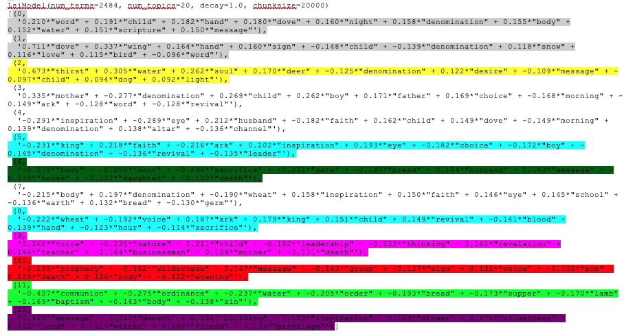
Figure 1 shows a visualization of the findings of the Latent Dirichlet Allocation Model.

Visualization was performed using the python pyLDAvis package, https://pypi.org/project/pyLDAvis/1.0.0/

The main topic associated with 1965-1212_Communion is highlighted in red. Note that the topic numbers in the visualization are different from those where the models are printed out (I have noticed this on the web too). There are some overlaps among topics (which require further work). There is one strongest topic in the north-west and a number of tiny topics towards the east.

The main topic associated with 1965-1207_Leadership and 1965-1031y_Leadership is shown in Figure 2.

The main topic associated with 1965-0919_Thirst is shown in Figure 3.

The main topic associated with Noah’s dove (1965-1128z_OnTheWingsOfASnowWhiteDove) is shown in Figure 4.

Comparison of the 3 models using Topic Coherence

I used the technique of topic coherence to draw a comparison between the three models. This technique only works when comparing models based on the same dataset. As is evident from Figure 5, the LDA (Latent Dirichlet Allocation) model fared the best. After it came the HDP (Hierarchical Dirichlet Process) and then the LSI (Latent Semantic Indexing) model.

Network Analysis of the LSI Topic Model

I have visualized the topic model of the LDA model above. For the visualization of a network model I will use the LSI topic model. Although this is the weakest model, it was easiest to construct its incidence matrix because it has the fewest number of topics (13). For the connection of each of the topics the top 10 words were used from the topic model. The incidence matrix is in the file IncidenceMatrixLSI.csv. The network analysis of the LSI topic model is in the file TextMiningProject-graph.ipynb.

After reading in the incidence matrix, the NaN’s are replaced with zeros and the data is prepared for consumption by the python-igraph package. A bipartite graph is created with 88 vertices and 142 edges. Names are provided for the vertices from the row and column names of the incidence matrix. Figure 6 shows the bipartite graph of the LSI topic model.

The red vertices represent the topics and the blue vertices the words.

Next, the bipartite graph was projected into a graph for topics and a graph for words. Figure 7 shows the topic graph for the LSI topic model.

Figure 8 shows the word graph for the LSI topic model.

Conclusion and Further Work

Overall, I am impressed by the possibilities of topic modeling. Although the models I derived were not adequate enough for my purposes, I think it might not require too much more work to make them usable. I would like to pursue this idea further and apply it in the areas of semantic search, tagging of each sermon with its highest-probability topics, and tracking of topics over time by means of dynamic topic models (Blei 2012).

References/Bibliography

Cloverdale Bible Way: https://bibleway.org/

Message Hub: http://www.messagehub.info/en/messages.do?show_en=true

Lev Konstantinovskiy: https://www.linkedin.com/in/levkonst/?originalSubdomain=uk

Blei, D.M. Probabilistic Topic Models, 2012.

pyLDAvis python package: https://pypi.org/project/pyLDAvis/1.0.0/